
Last week we covered traceroutes, and why you should gather data on both the forward path and the reverse path. This week we are looking at MTR, why you should use it, and how to interpret the results.
‘traceroute’ is a very handy tool, and it exists on most operating systems. If it isn’t there by default, there is almost undoubtedly a package you can install, or at worst, source code available to download and compile for your particular OS. Its one downfall is that it does one task, providing the path. Sometimes that data isn’t enough on its own, you need to see the path over time and observe the situation as it stands with an average view.
Enter “MTR”, initially “Matt’s Trace Route” and since renamed “My Trace Route” is a tool that has existed for Unix systems for over 17 years. It has several advantages over the traditional traceroute, and is preferred by many because of them. It will run multiple traces sequentially, and provide the results as it goes, telling you what percentage of packets have been lost at any hop, some latency statistics per hop (average response time, worst response time, etc), and in the event the route changes while the trace is in progress it will expand each hop with the list of routers it has seen. MTR is available for most Unix systems via their package managers or by a source download. An MTR clone is available for Windows called WinMTR.
Let’s give a quick overview of how traceroute works. First it sends out an ICMP Echo request, with a TTL of 1. Whenever a request passes through a router it will decrement the TTL by 1 and if/when the TTL on a packet reaches 0, the expectation is that the router will generate an ICMP Type 11 packet in return, or a Time Exceeded. Therefore when traceroute sends the first packet, with a TTL of 1, it expires at the first router it encounters, and the packet that is returned contains enough information that traceroute knows the IP address of the first hop, and it can use a reverse DNS lookup to get a hostname for it. Then it will send out another ICMP Echo request with a TTL of 2, this packet will pass through the first hop, where the TTL is decreased to 1, and then expires at the second hop. This carries on until either the maximum TTL is reached (typically 30 by default) or the destination is reached.
![]()
In this example, the red line is TTL=1, the green line is TTL=2, the orange line TTL=3 and the blue line TTL=4, where we reach our destination and the trace is complete.
This is where we start to encounter issues, because in the land of hardware routers there is a distinct difference in how the router handles traffic for which the router itself is the destination (e.g. traffic TO the router) and how it handles traffic for other destinations (traffic THROUGH the router). In our example above, the router at the first hop needs to receive, process, and return the packet to the origin. However, the other three packets it doesn’t need to look at, it only needs pass them on. From a hardware perspective they are handled by two entirely different parts of the router.
Cisco routers, and the other hardware vendors, typically have grossly underpowered processors for performing compute tasks, most under the 2GHz mark and many older routers still in production environments are under 1GHz CPUs. Despite the low clock speed, they remain fast by using hardware. Unfiltered traffic which only passes through the router is handled by the forwarding or data planes. These are updated as required by the control plane, but beyond that they are able to just sit back and transfer packets like it was their purpose (hint: it was their purpose).
That significantly reduces the load on the CPU, but it will still be busy with any number of tasks from updating the routing tables (any time a BGP session refreshes, the routing table needs to be rebuilt) to processing things like SNMP requests to allowing administrators to log in via Telnet, SSH or the serial console and run commands. Included in that list is processing ICMP requests directed to the router itself (remember, ICMP packets passing through the router aren’t counted).
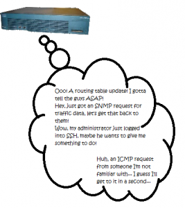
To prevent abuse, most routers have a Control Plane Policy in place to limit different kinds of traffic. BGP updates from known peers are typically accepted without filter, while BGP packets from unknown neighbors are rejected without question. SNMP requests may need to be rate limited or filtered, but if they’re from a known safe source, such as your monitoring server, they should be allowed through. ICMP packets may be dropped by this policy, or they may just be ratelimited. In any case, they CPU tends to consider them a low priority, so if it has more important tasks to do then they will just sit in the queue until the CPU has time to process them, or they expire.
Why is this important? Because they play a large role in interpreting an MTR result, such as the one below:
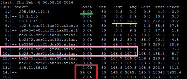
The first item is the green line. For some reason, we saw a 6% loss of the packets that were sent to our first hop. Remember the difference between traffic TO a router and traffic THROUGH a router. We are seeing 6% of packets being dropped at the first hop, but there is not a “packet loss issue” at this router. All that we are seeing is that the router is, either by policy or by its current load, not responding or not responding in time to our trace requests. If the router itself were dropping packets, we’d see that 6% propagating through the rest of the trace.
The second item is the yellow line, notice how the average response time for this hop is unusually higher compared to those before it? More importantly, notice how the next hop is lower again? This is a further indication that issues you could misinterpret from MTR are not really issues at all. Again, like the green line, all that we see here is that the router at hop 3 is either, by policy or by current process load, too busy to respond as quickly as other hops, so we see a delay in its response. Again, traffic through the router is being passed quickly, but ICMP traffic to the router is being responded to much more slowly.
The pink box is, to me, the most interesting one, and this is getting a little off track. Here we see the traffic go from New York (jfk, the airport code for one of New York’s airports, LGA is another common one for New York devices) to London (lon). There are several fiber links between New York and London, along with some other east coast US cities, but it still takes time for the light to travel between those two cities. The speed of light through a fiber optic cable is somewhere around c/1.46 (where c is the speed of light in a vacuum, or 300,000km/s and 1.46 is the refractive index of fiber optic cable). The distance from New York to London is around 5575 km. So even if the fiber were in a straight line, the best latency we could expect between those two locations is 5575*(1.46/300,000)*1000*2 is about 54ms.
[notice]This is a simple calculation for guessing ideal scenarios. It is generally invalid to use it as an argument because a) fiber optic cables are rarely in a straight line, b) routers, switches and repeaters often get in the way, and c) most of these calculations are on estimates which err on the side of a smaller round trip time than a longer one.
The calculation is as follows:
$distancebetweentwocities_km * (1.46 / 300,000) * 1000 * 2
(or for you folk not upgraded to metric, $distancebetweentwocities_miles * (1.46 / 186,000) * 1000 * 2)
You take the brackets and calculate the estimated speed of light through the fiber, then multiply that by the distance between your two cities to calculate the estimated time in seconds, then multiply that by 1000 to get milliseconds, then multiply that by 2 to get your round trip time in ms.[/notice]
We can see from the trace that it takes closer to 70ms for the packet to go from New York to London, so we’re actually looking pretty good.
Back to the real results, we see in hops 13 and 15 that there is a 2% loss. Over 50 packets this is only 1, so it’s difficult to know for sure, but remembering what we said before about through vs. to, in this case it is possible that the packet lost at hop 13 was actually lost and not just dropped by the router. We also have a 24% drop at hop 14, so it’s possible that the packet lost at hop 13 was coincidental and the packet lost by 15 was actually lost at hop 14.
So there it is, interpreting MTR results. The core notes you should take away are these:
- If you see packet loss at a hop along the route, but the loss is not carried through remaining hops, it’s more likely a result of ICMP deprioritization at that hop, it’s almost certainly not an issue of packet loss along the path.
- The same applies to latency, if you are seeing increased latency at a single hop but the latency is not carried through the remaining hops, it’s more likely a result of ICMP deprioritization at that hop.
- If you’re submitting an MTR report to your ISP to report an issue, make sure you get one for the return path as well (see Part One, last week’s post).